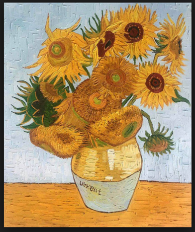
Machine learning (also called artificial intelligence or artificial neural networks) was originally designed to help better understand how the brain works. For example, how does the brain recognize images? Have a look at the image above, and describe what you see.
At the most basic level, it shows a vase sitting on a table next to a wall, and containing flowers (specifically, sunflowers). At the next level, many of you will have recognized it as one of Vincent van Gogh’s most famous paintings. This may have led you to thinking about poor Vincent’s tragic life and the fact he died penniless. Or you may have remembered going to an art museum and seeing the painting in person. How does the brain do all of this, often in a split second? Explaining how the image evokes memories is a very complex problem, but I will try to explain how a computer can recognize this picture as a vase containing flowers.
Santiago Ramón y Cajal, a Spanish neuroscientist who lived from 1852 to 1934, is often credited as the founder of neural network and machine learning research. He discovered the axonal growth cone and dendritic spines in neurons in the brain, and the fact that there were gaps between neurons that suggested that information could be transmitted between neurons by electrical signals. His detailed drawings of neurons inspired future generations of scientists to propose mathematical models of the neuron, which led to neural network and machine learning techniques.
The figure below shows a schematic diagram of a neuron, illustrating how the axon is fed by electrical signals from the dendrites into the cell body and then on to the axon terminal.
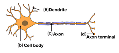
A schematic diagram of a neuron (courtesy Wikipedia)
The neuron was first quantified by Donald Hebb, a Canadian neuroscientist, in his book The Organization of Behaviour, published in 1949. Hebb stated: “When an axon of cell A is near enough to excite a cell B …, some growth or metabolic change takes place in one or both cells…” This is now called Hebbian learning, and in mathematical terms can be expressed as the connection between two neurons being proportional to the correlation of their activation values during learning. Here is a simple example:
Our brain records thousands of images daily, and although we cannot model how the billions of neurons in the brain store these images, consider the two neurons shown in the next figure: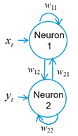
Each neuron is fed by a stream of inputs, which I write as xt for the first neuron, and yt for the second, where t means the time increment. Although we think of time as being continuous, in the machine learning approach, time is digitized into discrete values of a fraction of a second. Let’s only allow two inputs of either +1 or -1 (light and dark), so that the string of inputs could be:

The two neurons are also connected by weights written as wij, the weight between the ith and jth neurons, where if i = j, the weight is applied to the neuron itself. These weights can be arranged into a square matrix as follows:

Matrices are used in a type of mathematics called linear algebra, which is the basis of most machine learning techniques (see Strang, 2019). For those who have never studied linear algebra, I will do my best to explain in brief.
Since we only have two neurons with two states (+ or – 1, corresponding to light and dark), there are only four possible two-pixel (where a pixel is a single visible point) images, shown below:

We could label these images as WW, BW, WB, and BB, where W stands for white and B for black, and let’s give them the mathematical description

where the letter p stands for picture (or point on a two-dimensional graph), and the columns of two numbers are called vectors, the other main idea in linear algebra. Let’s look at the concept of “correlation” in Hebbian learning. We can correlate each of the pictures with itself by multiplying the transpose of the vector by the original vector, where transpose simply means to turn the vector from a column to a row. Mathematically, we can write:

Correlation has given us a matrix the same size as the weight matrix, with the following interpretation: the number in the upper left-hand corner is the correlation of the x value with itself, the number in the lower right-hand corner is the correlation of the y value with itself, and the numbers in the other two corners are the correlation of the x value with the y value.
We are now in a position to compute the full weight matrix that will allow our eye to distinguish which of the four images we ae are looking at. We simply sum the correlations of the four cases and multiply by what is called a learning rate. In this case, I will set the learning rate to one divided by the number of images. Using all four images gives us

The resulting matrix, with ones on the main diagonal and zeros elsewhere, is called the identity matrix and is the equivalent in linear algebra of one in arithmetic. What this means is that whenever this “eye” looks at a new image (remember, there are only four possible images), it multiplies the weight matrix by the new image to see if it recognizes the image. We can write:

For example, if we look at the black-white image, we will recognize it as the black-white image:

Visually, we can draw this as
![]()
It is obvious that all four images will be recognized. However, let’s say we had trained the eye with just the first and last image. Then, the weight matrix would be computed as follows:

Applying this set of weights to the second image gives

If we let 0 represent grey, we can interpret this visually as

In other words, the eye doesn’t recognize this image since it has never seen it before, and thus has no visual memory of it.
This two-pixel, black-and-white example is obviously much too simple to represent true vision. Let’s move to the next level of complexity, in which we still have two colours, but now we have four pixels. As seen below, this leads to a total of 16 2×2 images:
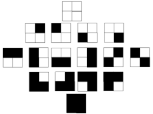
Mathematically, this means that the number of possible images for M colours with N pixels is MN, which for two pixels and two colours is 22 = 2×2 = 4 images and for four pixels with two colours is 24 = 2x2x2x2 = 16 images. We could write the above 16 pictures as matrices in the following way:

In machine learning, we also talk about “flattening” a two-dimensional image into a vector, so that we could also write the images as:

I could go through the same analysis for this four-pixel image as for the two-pixel image, but it still would not capture nearly the complexity of any reasonable picture. Let’s therefore consider the cartoon face shown below, which is on a 9×9 = 81-pixel grid, with three colours: white (+1), grey (0), and black (-1).
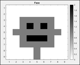
Mathematically, we can write this as the following 9×9 matrix:

But this is only one of the 381 = 4.434 x 1038 possible arrangements of three colours on a 9×9 grid. If you don’t use exponential notation, that is roughly 4,434 times a trillion-trillion-trillion number of pictures! Obviously, we must reduce the number of possible images or else the computational time to recognize this face would be the lifetime of the universe! To do this, a new type of machine learning technique called the Convolutional Neural Network, or CNN, has been developed. The term convolutional refers to the fact that two-dimensional convolutional filters, or kernels, are applied to the image to look for “features” that can be used to identify a particular picture. Three common kernels are the vertical (V), horizontal (H), and edge (E) kernels, which can be written in matrix format as shown below

The following three images show the application of a vertical (left panel), horizontal (middle panel), and edge (right panel) kernels to our face picture, where vertical, horizontal, and edge effects have been isolated.

But this doesn’t really help us, since the three images shown above all have the same number of pixels as the original image. To reduce the number of pixels, CNN uses a number of tricks, which are referred to as padding, striding, and pooling. Padding is used to widen the image being filtered, and striding is the number of pixels that are skipped as the filter moves across the image. The size of the resulting image (NxN) is given by the following formula:

In the three original filtered images, W = 9, K = 3, P = 1, and S = 1, so N = 9 (check the math), and the resulting image is the same size as the original. But if we change S to 2 and P to 0, and use the edge filter, the output is reduced to a 4×4 image shown on the right below. This image is different from the one on the left, but retains some of its features.

In pooling the image is divided into squares, and each square is averaged. For example, if we divide the 4×4 image on the above right into 4 2×2 squares, pool them, and then flatten the 2×2 matrix into a 4×1 vector, the result is as shown below:
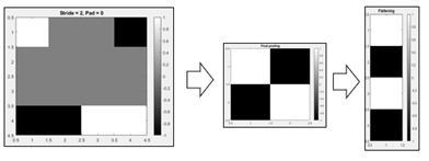
Notice that we have reduced a complex picture into a four-pixel result, which we have seen has only 16 possible interpretations.
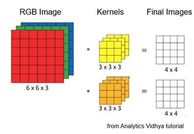
Of course, we have been talking only about black/white/grey images. What about full-colour pictures? In this case, we can input the image using the RGB (red/green/blue) decomposition shown below. The red, green, and blue images add an extra dimension to our matrix, which is now called a tensor. This led to the TensorFlow program from Google, which is used in the development of new machine learning programs. Note in the figure below that the kernels themselves are in tensor format.
In the interest of time and space today, I have focused on just one type of machine learning technique, which is called unsupervised Hebbian learning. The CNN approach uses the supervised learning approach, in which labels are attached to the desired output images. This is shown in our final image below, where CNN is trying to decide if the input picture is a dog, cat, boat, or bird (proving that computers have a long way to go to catch up to humans!).

In the above figure, the term ReLU refers to a type of nonlinear function that is used in supervised learning algorithms. For more details on this, you can refer to the book by Goodfellow et al. (2016) Perhaps this will also lead me to a more advanced tutorial.
References
Goodfellow, I, Bengio, Y., Courville, A., 2016, Deep Learning, The MIT Press.
Hebb, D.O., 1949: The Organization of Behaviour: A Neuropsychological Theory, New York, Wiley.
Strang, G., 2019, Linear Algebra and Learning from Data, Wellesley-Cambridge Press.
(Brian Russell – BIG Media Ltd., 2023)
