Bayes’ Theorem and the probability of having cancer

(With files from Laurie Weston)

Let’s suppose that your medical doctor finds something of concern and suspects that you may have cancer. Your doctor’s first step is to send you for some type of non-invasive test, such as an X-ray or MRI. A few days later, you receive a phone call from your doctor, and you get the news you have been dreading. Your test is positive.

So, how concerned should you be? Although you should be quite concerned, it turns out that you have less than 10% chance of having cancer. This may be hard to believe, but the reason is that cancer tests are never 100% reliable. We will see how that uncertainty translates into a probability that can be determined mathematically.

In this article, I will explain how we can come up with the value of the probability that you have cancer given that you have a positive test. This method involves a statistical idea that was developed by the Reverend Thomas Bayes in the 18th century and is now referred to as Bayes’ Theorem.

The first thing to understand is that statistics always involves data; the more the better. Chart 1 shows a grid of 1,000 people, where the blue figures represent people without cancer, and the red figures represent people with cancer. This grid could represent the crowd at a football stadium or the distribution of individuals in a city. The red figures are drawn in random order to indicate that cancer is generally spread throughout the community. If you count the red people, you will see that there are 10, meaning that 10 out of 1,000, or 1%,[1] of this population has cancer.[2]

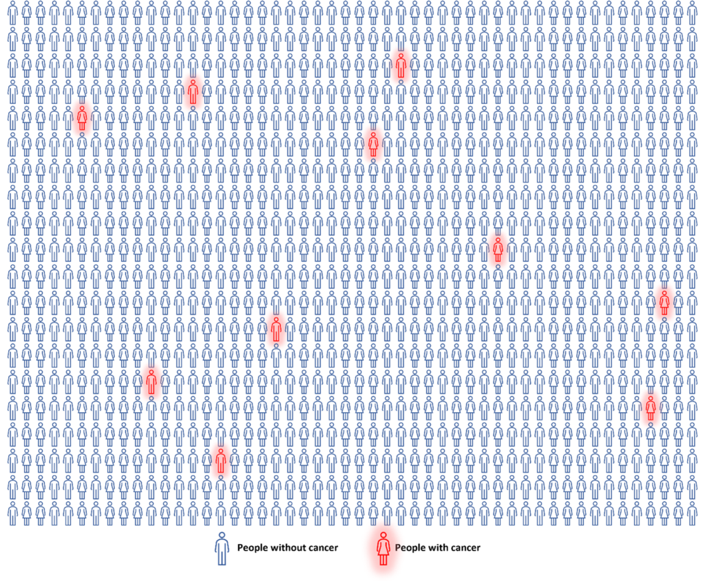
Chart 1: A group of 1,000 people, where the blue figures indicate people without cancer, and the red figures indicate individuals with cancer.

Chart 2 shows the same group of people, but after one of the typical medical tests for cancer. The reliability of a cancer-screening test is called its sensitivity. Depending on the test and the stage of cancer, there can be a wide range of sensitivity.[3]  Let’s say, for the sake of this mathematic exercise, that the sensitivity of this test is 80%, which would mean that 8 out of the 10 people who have cancer would get a positive test result, and the other 2 would come back negative. Conversely, assuming the negative test outcome has a reliability factor (called “specificity”) of 90%, out of 990 people who do not have cancer, 90% (891) would be correctly informed, and 10% (99) would be told they have cancer when they do not. The total number of people receiving a positive test result would therefore be 107: the sum of the 8 who do have cancer and the 99 who do not. The yellow figures in Chart 2 represent everyone who tested positive for cancer (107) and the green figures represent the remaining total number of people who tested negative for cancer (893).

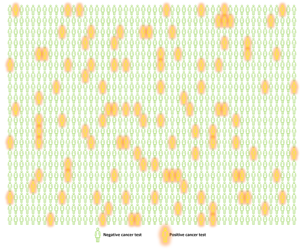
Chart 2: The same group of 1000 people as in Figure 1, where the yellow figures indicate people who tested positive for cancer and the green figures indicate individuals who tested negative for cancer.

A third plot combines the two previous, with four sets of coloured figures representing the four outcomes. The blue figures represent the situation in which the person has both a negative test and is cancer free. This is called a true negative. The red figures represent the scenario in which the person has a positive test and has cancer. This is called a true positive. The yellow figures represent the situation where the person has a positive test but does not have cancer. These are called false positives. Finally, the green figures represent the scenario in which the person has a negative test but has cancer. This is called a false negative.

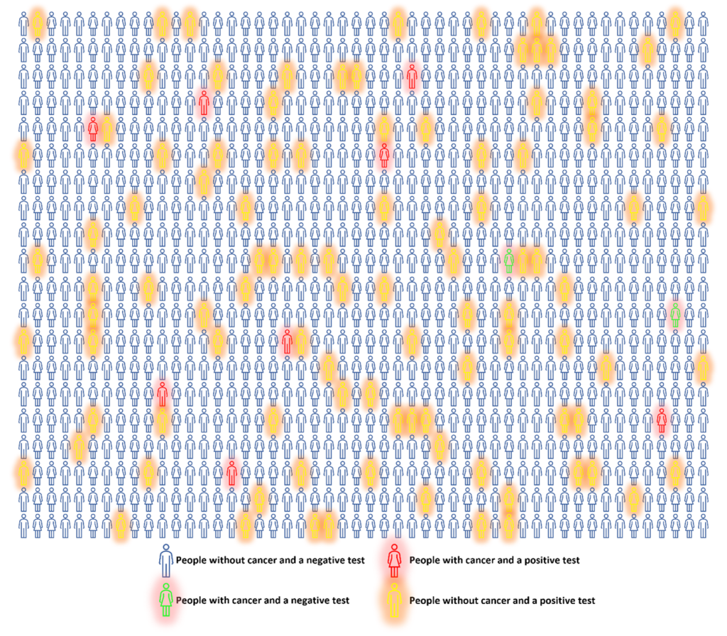
Chart 3. The same group of 1,000 people as in Charts 1 and 2, where the blue figures indicate true negatives, the red figures indicate true positives, the yellow figures indicate false positives, and the green figures indicate false negatives.

I started with Charts 1 through 3 to give you a visual image of 1,000 people with and without cancer. This is obviously a very inefficient way to analyse data. What if the study was on 10,000 people? A more efficient way is to create a summary table of the data, as shown below in Table 1.

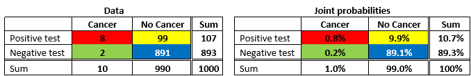
Table 1. Cancer and test incidences for 1,000 people, assuming imperfect test results, colour coded for true positives (red box), true negatives (blue box), false positives (yellow box) and false negatives (green box). The data is shown on the left, and the percentages of each occurrence (joint probabilities) are calculated on the right.

Table 1 (left) contains all the information shown in Charts 1 through 3, but in a much more compact form. It has been colour coded to match Chart 3, where true positives are in the red box, true negatives are in the blue box, false positives are in the yellow box and false negatives are in the green box. If you add these four numbers together you get the total population of 1,000 people, which is also given in the lower righthand box in the table. If you divide each of these numbers by 1,000 and convert from decimal to a percentage, you get the probability of each of these results shown in Table 1 (right). That is, each person in the group has a 0.8% probability of having a true positive, an 89.1% chance of having a true negative, a 0.2% chance of having a false negative, and a 9.9% chance of having a false positive. If you add these numbers together, you get 100%, which is saying that everyone must fall into one of the four categories. To be more precise, we will call these the joint probabilities. This is the probability that you jointly have one outcome from a row and one outcome from a column – e.g., a negative test and have cancer.

But notice there is more information in Table 1 than just these four numbers. At the right of the two rows of numbers and at the bottom of the two columns are their sums. These are shown in Table 2, which is the same as Table 1, except for the coloured cells.

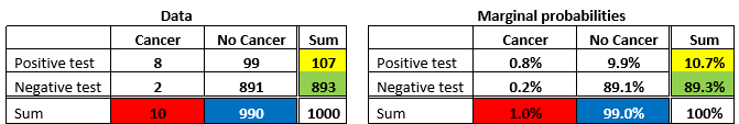
Table 2. Cancer rates for 1,000 people, assuming imperfect test results. The sums of each row and column are colour coded for positive tests (yellow), negative tests (green), individuals with cancer (red), and individuals without cancer (blue). The percentages of the total are shown as marginal probabilities on the right.

The green and yellow sums of the rows in Table 2 (left) correspond to the people shown in Chart 2, where 107 had positive test results and the remainder, 893, had negative test results. The red and blue sums correspond to the people in Chart 1, where 10 had cancer and 990 were cancer free. Adding the column sums and row sums gives 1,000 again, as it should. Dividing these sums by 1,000 and converting to a percentage gives us the marginal probabilities shown in Table 2 (right). So, we see that 1% of the population has cancer and 99% does not. Also, 10.7% of the population got a positive test result, and 89.3% got a negative result. Again, adding both the column percentages and row percentages will give 100% (you either have cancer or don’t, and you either have a positive result or a negative result). Let’s now look at a third type of probability, called conditional probability, which is the most important part of Bayes’ Theorem.

We already know that in a random group of 1,000 people, you have a 10 in 1000, or 1% chance of having cancer. But, if you are one of the people who receive a positive test result, what are the chances you have cancer? Given that we know only 8 (true positives) of the 107 who tested positive actually have the disease, the answer is 8/107, or only 7.5%. This calculation is called the “conditional” probability, defined as the probability of one of the two possibilities of each event[4] happening, given that one of the possibilities of the other event has already happened; in this case, the probability of having cancer, given that you have received a positive test result (highlighted in Table 3 left). Switching the order of these events, the probability of having a positive test result, given that you have cancer, is 8 true positives out of the 10 that do have cancer, or 80% (highlighted in Table 3 right). All of the conditional probabilities for each possible situation are shown in Table 3.

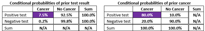
Table 3: Conditional probabilities, given a certain test result (left), or given the existence of cancer (right).

How does Bayes’ Theorem give us an even more straightforward way of interpreting the probabilities we found using Tables 1, 2, and 3?

Remember that using the numbers in the three tables, we defined three types of probability: joint probability, marginal probability, and conditional probability. Thomas Bayes noticed the relationship between these three probabilities. What he found was both simple and profound:

“The conditional probability of having cancer given that you have a positive test result is equal to the conditional probability of having a positive test given that you have cancer multiplied by the marginal probability of having cancer and divided by the marginal probability of a positive test.”

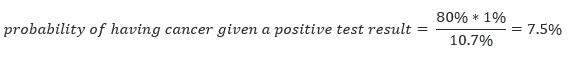
Phew! That might not sound so simple and profound to most people, but, often, mathematical concepts are much more elegant in their natural state: an equation. In Bayes’ Theorem, the conditional probability of having a positive test result given that you have cancer (80%) is called the likelihood (how likely are you to test positive if you have cancer?), the marginal probability of having cancer, which is 1%, is called the prior (what is your prior probability of having cancer?), and the marginal probability of having a positive test, or 10.7%, is called the evidence (what is your prior probability of testing positive?). Using these terms, Bayes’ Theorem can be written as

In the real world, we do not have the benefit of Charts 1 and 3 because we do not know in advance who has cancer (that is why we do the testing); we only have the information illustrated in Chart 2: positive and negative test results. The “posterior” that can be calculated from this formula therefore refers to exactly what we want to know; the probability of having cancer, given that we have received a positive test. Filling in the numbers from the appropriate boxes in the tables gives:

The beauty of this method is that if any of the numbers change with updated studies or other sources, the calculation can simply be redone using only the basic arithmetic in the Bayes’ Theorem equation. For example, if new scientific insights change the prior probability of having cancer from 1% of the general population to 5%, the new probability of having cancer if you receive a positive test is easily calculated (29.6%).[5]

Math can give us the right tools for the job (sometimes several related jobs) if we know where to look and how to apply those tools. Bayes’ Theorem is a versatile tool that can be used to simplify complex concepts and statistical relationships. The example in this article demonstrated the power of a mathematical method to help us better understand things in our largely uncertain everyday life.

[1] I have rounded up from the actual 0.6% to 1% so we don’t have partial people in our 1,000-person sample exercise.

[2]Projected estimates of cancer in Canada in 2020, Darren R. Brenner PhD, Hannah K. Weir PhD, Alain A. Demers MSc PhD, Larry F. Ellison MSc, Cheryl Louzado MSc MHSc, Amanda Shaw MSc, Donna Turner PhD, Ryan R. Woods PhD, Leah M. Smith PhD; for the Canadian Cancer Statistics Advisory Committee, CMAJ 2020 March 2;192:E199-205. doi: 10.1503/cmaj.191292 (accessed June 30, 2021).

[3] A multi-cancer detection test: focus on the positive predictive value, C. Fiala, E.P. Diamandis, Annals of Oncology, Vol 31, Issue 9, P1267-1268, September, 2020 DOI: (accessed July 1, 2021).

[4] I am using the term “event” the way a statistician would use it. That is, having or not having cancer is one event, and having a positive or negative test result is the other event.

[5] For you sharp-eyed readers, the reason this result is not simply 5 times 7.5% is because the denominator (the evidence) also changes when the prior changes.