Do we ever use the mathematics we learn in school? Does it matter? These questions are pondered by most students at one time or another, and perhaps surprisingly, even by mathematicians. In a paper called “The Unreasonable Effectiveness of Mathematics in the Natural Sciences” written in 1960 by physicist Eugene Wigner, the author marvels at the importance and practicality of mathematics in the physical sciences. Wigner notes that the significance of math goes far beyond expectations, sometimes far beyond the original intent in its creation, and often surprises its practitioners with unexpected internal connections.[1]He is at a loss to explain why its use is so exceptional. But exceptional, mathematics is.
I agree with Wigner and would add that mathematics is also very useful in everyday life, even if we do not always notice it explicitly. Like so many things in this wide world of ours, mathematics needs an open mind and open eyes to be fully appreciated. Even so, mathematics is a very large subject, so in this article I will focus on one ubiquitous mathematical function – the exponential – and show how useful it is in day-to-day life, in science and mathematics, and how it has some unexpected interconnections.
Compound interest and the exponential function
To introduce the exponential, let’s start with a common investment problem. Suppose you invest $10,000 at an interest rate of 5%, compounded annually. To compute the amount of interest you would earn after n years, the formula is given by
I = [P(1+i)n] – P, (1)
where I is the total interest earned in n years, P is the principal, and i is the interest rate as a decimal value. In equation (1), the exponential part is (1+i)n, which is read as (1+i) raised to the nth power. Since n is an integer, this simply means we multiply (1+ i) by itself n times. Let’s say we invest for n = 3 years. Then, the interest in our case would be
I = [$10,000(1.05)3] – $10,000 = [$10,000(1.158)] – $10,000 = $1,580
That is, after three years, you would have made $1,580 on your original investment. (Notice that I rounded to 1.158 in the above calculation; if you use the exact value, you only get $1576.25.) This seems quite reasonable, but let’s see what happens over a longer period. Figure 1 below shows the same investment over 50 years. As you can see, your original investment will have returned $104,674 in interest over 50 years.
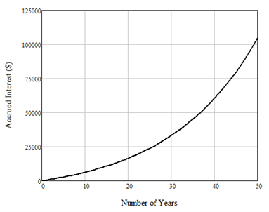
Figure 1: Compound interest on $10,000 at a 5% interest rate, compounded annually.
The exponential and your home’s value
As pointed out by my fellow geoscientist friend Lee Hunt, this same equation can be used to decide whether it is better to invest in real estate or in the bank. Let’s say you bought a property and held it for 20 years, then sold it for double what you paid for it. You would be quite happy with that. But by letting (1+i)20 = 2 and inverting for i (that is i = 21/20 – 1), you would find that you would have made as much money with your original investment at just a 3.5% interest rate!
Exponentials and the spooky, time-symmetric, natural base of ‘e’
The rising curve you see in Figure 1, called an exponential curve, has applications throughout all of mathematics and science[2]. In mathematics, the exponential curve is written as y(t) = bt, where b is called the base and y(t) is a function of continuous time, or t. The inverse of the exponential is the logarithm, which is written t = logb(y). As a simple example, if b = 10 and t = 2, then y = 100 and t = log10(100) equals 2. Although any number can be used as the base, the number that is preferred by mathematicians is the “natural base” e, a transcendental number that cannot be represented by a finite number of decimals, although it is often truncated to the value 2.718. Its inverse is called the natural logarithm, written loge or simply ln. If you haven’t studied calculus or trigonometry, this may not be familiar to you. In simple terms, calculus is about the slopes of curves, called derivatives, and the areas under curves, called integrals. Here is the amazing result that leads to e: if the base of an exponential equals e, its derivative is equal to itself. Using derivative notation, the equation is det/dt = et. Figure 2 shows the two exponential curves et and![]() , where negative time indicates the past, and positive time indicates the future. Strang[3]states that this is the one idea that really makes Calculus unique from any other branch of mathematics.
, where negative time indicates the past, and positive time indicates the future. Strang[3]states that this is the one idea that really makes Calculus unique from any other branch of mathematics.
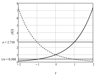
Figure 2: The exponential curve et (solid line) and its inverse e-t (dashed line).
The symmetry of the two curves in Figure 2 is remarkable. Both cross the y axis at a value of 1 for t = 0 since any function raised to the 0th power equals 1. The value is e for et at t = +1 and for e-t at t = -1, and the value is 1/e for et at t = -1 and for e-t at t = +1. The exponential curves look the same for any base b, with the exception that the horizontal lines on the plot would now be at b and 1/b.
Exponential population growth
In science, the natural exponential curve is found in growth problems such as population growth where it is the solution of the simplest differential equation. In a differential equation, we are asked to find the function that has a given derivative rather than the derivative of a given function.[4] For population growth, this equation is
dy(t)/dt = ay(t), (2)
where a is a scaling term that I will explain shortly. Since we have already seen that the function that is the derivative of itself is the natural exponential curve, this is obviously the solution to y(t), modified by two scaling constants to give y(t) = ceat, where a controls the steepness of the curve and c is the value at t = 0. If this all sounds too theoretical, let’s apply it to population growth in Canada. Figure 3 shows population growth in Canada from 1960 to 2010, where the open circles indicate the population, in millions, for each year. The curves represent three different exponential curves fitted with different values of a in the equation population(t) = p0eat, where p0 was the population in 1950. That is, c = p0.
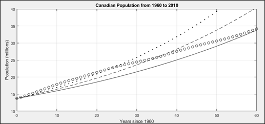
Figure 3: Population growth in Canada from 1950 to 2010, where the open circles represent the population, the solid line is an exponential fit with a = 0.015, the dashed line is an exponential fit with a = 0.018, and the dotted line is an exponential fit with a = 0.021.
A better model for population growth?
It is obvious from Figure 3 that Canada is not undergoing pure exponential growth since none of the curves fits the population trend. If we were experiencing exponential growth (for example, like the dotted line), this would eventually lead to a situation in which the population becomes unsustainable. In any population, something always happens to restrict the growth, be it disease or famine or out-migration. In mathematics, this is often called the predator-prey problem because an abundance of prey will always attract more predators. Luckily for us, we don’t face predators in our everyday lives, but we do have modifying factors such as disease, variable birth rates, immigration, and so on. Modelling this type of population growth is done by mathematicians through adding a second term to the earlier differential equation, which depends on the square of the population growth[5], or
dy(t)/dt = ay(t) – by(t)2, (3)
This is a much more difficult equation to solve than Equation 2, but it has a beautiful solution called the logistic function. For a = b = 1, the logistic function is written
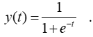 (4)
(4)
The logistic function is shown in Figure 4. Looking at the figure and Equation 4, notice that the curve equals ½ at t = 0 (since e0 = 1) but flattens to 1 for large positive values of t (since e-t goes to 0) and to 0 for large negative values of t (since e-t goes to infinity). The logistic function, often called the “squashing function”, is used as the nonlinear function of preference in many machine-learning applications[6](I’ll save this for a later article).
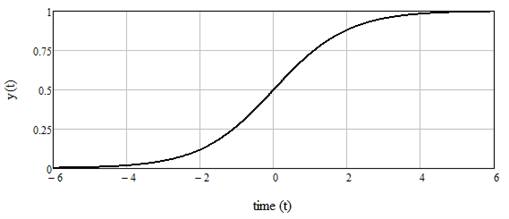
Figure 4: The logistic function from equation 4.
In essence, the logistic function considers a ceiling for growth.
The full solution to equation (3) for arbitrary values of a and b is given by
![]() (5)
(5)
where c = a/y(0) – b.[7]In our population problem, y(0) is the population in 1950, and Figure 4 shows the logistic equation fit where a = 1.04 x 10⁻⁹ and b = 1.87 x 10⁻⁹.
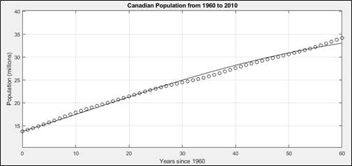
Figure 5: Population growth in Canada from 1950 to 2010, where the open circles represent the population, and the solid line is the logistic fit. Note how much better this fit is than the exponential fits of Figure 3.
The exponential’s relationship to the bell curve that everyone knows and loves
Finally, I will introduce a new exponential function by simply squaring the term t in the inverse exponential function, giving us what is called the Gaussian function, or
![]() (6)
(6)
The Gaussian function is shown in Figure 5. As seen in the figure, the squaring operation has made the curve symmetric around zero and smoothed out the top of the function. The Gaussian curve has a maximum value of 1 and, although it appears to go to 0 at both ends, it never reaches zero, but very small values close to zero.
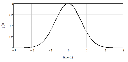
Figure 6: The Gaussian function from Equation 6.
The Gaussian curve is the classic “bell-shaped” curve, and leads us to the Gaussian, or Normal, distribution in statistics[8]. To understand the Gaussian distribution, we need two ideas from statistics, the mean, or μ, which is the average of a set of measurements, and the variance, or σ2, which is the average squared deviations of the measurements around their mean. The square root of the variance, or σ, is called the standard deviation. The Gaussian function in Equation 6 becomes the Gaussian distribution by subtracting the mean from each value (x is usually used instead of t in statistics), dividing by twice the variance and multiplying by a factor that ensures the area under the curve equals 1. The final equation is
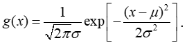 (7)
(7)
To make this equation more readable, I have used the notation exp in place of e, which is common practice in mathematics. The appearance of the square root of π, or pi, in the scaling factor is one of those magical mathematical results Wigner marvels about in his article.
Figure 7 shows two Gaussian distributions, both with a mean of 2, but one with a standard deviation of 1 and the other with a standard deviation of ½. Notice that as the standard deviation increases, the curve flattens out. Conversely, as the standard deviation decreases, the curve becomes more of a peak.
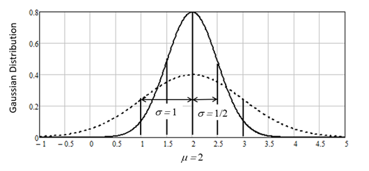
Figure 7: The Gaussian distribution from Equation 7 for two separate curves, both with a mean of 2 but the dashed curve with a standard deviation of 1 and the solid curve with a standard deviation of ½.
An example from earth properties
This is the theory, but how does it work in practice on real data? Figure 8 shows the probability distribution of a set of 1,188 geophysical measurements taken in a well log. The measurement is the ratio of the compressional velocity Vp to the shear velocity Vs of a reservoir rock, which is often an indication of its fluid content. From this distribution, it is found that the mean is 1.75 and the variance is 0.15.
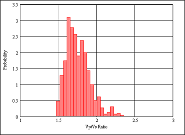
Figure 8: The probability distribution of a set of 1,188 geophysical measurements taken in a vertical well log, where the mean is 1.75 and the variance is 0.15.
In Figure 9, I have superimposed the Gaussian distribution from Equation 8 using the measured mean and standard deviations, which are shown on the plot. Notice that the fit is quite good but some of the lower and higher values stick up above the curves. Thus, the Gaussian distribution is not a perfect model for these data. For example, the small group of points centered on a value of about 2.2 may represent a second, smaller Gaussian distribution of points.
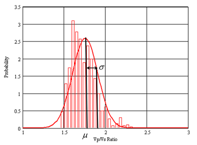
Figure 9: The red line shows the Gaussian distribution curve superimposed on the probability distribution from Figure 8, where the mean and standard deviation are also shown.
This concludes my overview of the “ubiquitous exponential”. I showed how one simple function leads us to the concepts of compound interest, population modeling, machine learning, and Gaussian statistics. These key curves were the exponential curve itself, the logistic function, and the Gaussian. Coming back to the question of whether we ever use the mathematics we learn in school … we may not all learn that math, but it is all around us, present and acting, and is a key, lens, and translator needed to understand this ever-changing world.
References
[1] Wigner, Eugene, 1960, The Unreasonable Effectiveness of Mathematics in the Natural Sciences, Communications in Pure and Applied Mathematics, V. 13, No I
[2] Courant, R., H. Robbins, and I. Stewart, 1996, What is Mathematics?, 2nd Revised Edition: Oxford University Press.
[3] Strang, Gilbert, 2010, Calculus: Wellesley-Cambridge Press.
[4] Strang, Gilbert, 2014, Differential Equations and Linear Algebra: Wellesley-Cambridge Press
[5] Strang, Gilbert, 2014, Differential Equations and Linear Algebra: Wellesley-Cambridge Press
[6] Bishop, C.M., 2006, Pattern Recognition and Machine Learning: Springer
[7] Strang, Gilbert, 2014, Differential Equations and Linear Algebra: Wellesley-Cambridge Press
[8] Davis, J.C., 1986, Statistics and Data Analysis in Geology, 2nd Edition: John Wiley and Sons Inc.
(Brian Russell – BIG Media Ltd., 2022)